Learning Neural Causal Models with Active Interventions

• TL;DR:
  We propose to augment neural causal discovery methods with the ability to actively intervene. Therefore, we introduce Active Intervention Targeting (AIT), an adaptive intervention design technique for the batch-wise acquisition of interventional samples. AIT enables a quick identification of causal structure of the underlying data-generating process.
  Differentiable Causal Discovery

  Active Learning

  Experimental Design
• Please note that references are currently removed for readability. Please see the full-print on ArXiv for a complete version.

Why Active Neural Causal Discovery?

Inferring causal structure from data is a challenging but important task that lies at the heart of scientific reasoning and accomanyping progress. Recently, there has been a surge in interest in differentiable causal structure learning with neural networks, also known as neural causal discovery. These methods propose to avoid a discrete search over the combinatorial solution space by treating it as an optimization problem with smoothly differentiable parameters. The set of neural parameters embodies a neural causal model $\mathcal{N}$ that represents parameters of both structural and functional nature. Structural parameters express the belief about the graph structure through a distribution over graphs, for example with a soft-adjacency matrix. On the other hand, functional parameters characterize the conditional probability distributions of the factorized joint distribution of a directed graphical model. Overall, such models offer promising abilities with respect to generalization and fast adaptation.

Existing neural causal discovery methods focus on fixed datasets of either observational or fused (observational and interventional) nature. While having access to interventional data can significantly improve the identification of the underlying causal structure, the improvement critically depends on the nature of the experiments and the number of interventional samples available to the learner. In addition, interventions tend to be costly and can be technically impossible or even unethical. Hence it is desirable for an agent to conduct active interventions to recover the underlying causal structure in an adaptive and efficient manner. While a large body of work has addressed this need based on non-differentiable frameworks, existing work in neural causal discovery has not yet focused on incorporating active interventions.

In this work, we propose to augment neural causal discovery methods with the ability to actively intervene. Therefore, we introduce Active Intervention Targeting (AIT), an adaptive intervention design technique for the batch-wise acquisition of interventional samples. AIT can be easily incorporated into any neural causal discovery method which provides access to structural and functional parameters. In AIT, we decide where to intervene by computing a score for all possible intervention targets (over a single or multiple variables). This score provides us with an estimate how informative an intervention at that target would be with respect to the current evidence. For a set of hypothesis graphs sampled from the structural belief and a fixed intervention target, we apply the intervention on all hypothesis graphs and generate hypothetical samples through an ancestral sampling process based on the functional parameters. This allows us to compare statistics of the post-interventional sample distributions across the hypothesis graphs. We conjecture (and empirically show) that interventions that do not agree across different hypothesis graphs contain more information about the causal structure and hence enable more efficient learning.

• Contributions:
  We propose an intervention design method (single and multi-target) which identifies the underlying graph efficiently and can be used for any differentiable causal discovery method. We examine the proposed intervention-targeting method across multiple differentiable causal discovery frameworks in a wide range of settings and demonstrate superior performance against established competitive baselines on multiple benchmarks from simulated to real-world data. We provide empirical insights on the distribution of selected intervention targets and its connection to the topological order of the variables in the underlying data-generating distribution.

Structural Causal Models and Interventions

• Structural Causal Model (SCM) and Causal Factorization:
  A SCM is defined over a set of random variables $X_1, ..., X_N$ and a directed acyclic graph (DAG) $G=(V,E)$ over variable nodes $V\in\{1,...,N\}$. The random variables are connected by edges in $E$ via functions $f_i$ and jointly independent noise variables $U_i$ through $$ \small X_i \:= f_i(X_{pa(i)}, U_i) $$ where $X_{pa(i)}$ are parents in $G$, and directed edges in the graph represent causation.The conditionals $P(X_i|X_{pa(i)})$ define the conditional distribution of $X_i$ given its parents. This characterization entails a factorization of the joint observational distribution, also known as causal factorization: $$ \small P(X_1, \ldots, X_N) = \prod_{i=1}^{N} P(X_i|X_{pa(i)}) $$
• Interventions:
  Interventional settings represent the system under different perturbations and therefore affect the observed joint distribution. Specifically, an intervention on $X_i$ changes the conditional distribution of $P(X_i|X_{pa(i, \mathcal{G})})$ to a different distribution, hence affecting the outcome of $X_i$. Interventions can be hard (perfect) or soft (imperfect).
  
  Hard interventions entirely remove the dependencies of a variable $X_i$ on its parents $X_{pa(i, \mathcal{G})}$, hence defining the conditional probably distribution of $X_i$ by some $\tilde{P}(X_i)$ rather than $P(X_i|X_{pa(i, \mathcal{G})})$.
  
  Soft interventions are a more general form, where the intervention changes the effect of the parents of $X_i$ on itself by modifying the conditional distribution from $P(X_i|X_{pa(i, \mathcal{G})})$ to an alternative $\tilde{P}(X_i|X_{pa(i, \mathcal{G})})$.
  
  Interventions can be performed simultaneously on multiple variables of the systems. We denote the set of affected variables as \emph{interventional target set} $I \subseteq V$. Given such a set $I$ of size $|I|=k$, the joint distribution over all variable of the interventional setting for the general case of soft interventions is given by: \[ \small \tilde{P}(X_1, ..., X_N | do(I)) = \underbrace{\prod_{X_i \in V \setminus I} P(X_i|X_{pa(i, \mathcal{G})})}_{unperturbed} \hspace{2mm} \underbrace{\prod_{X_i \in I} \tilde{P}(X_i|X_{pa(i , \mathcal{G})})}_{perturbed} \]

How does Neural Causal Discovery from Fused Data work?

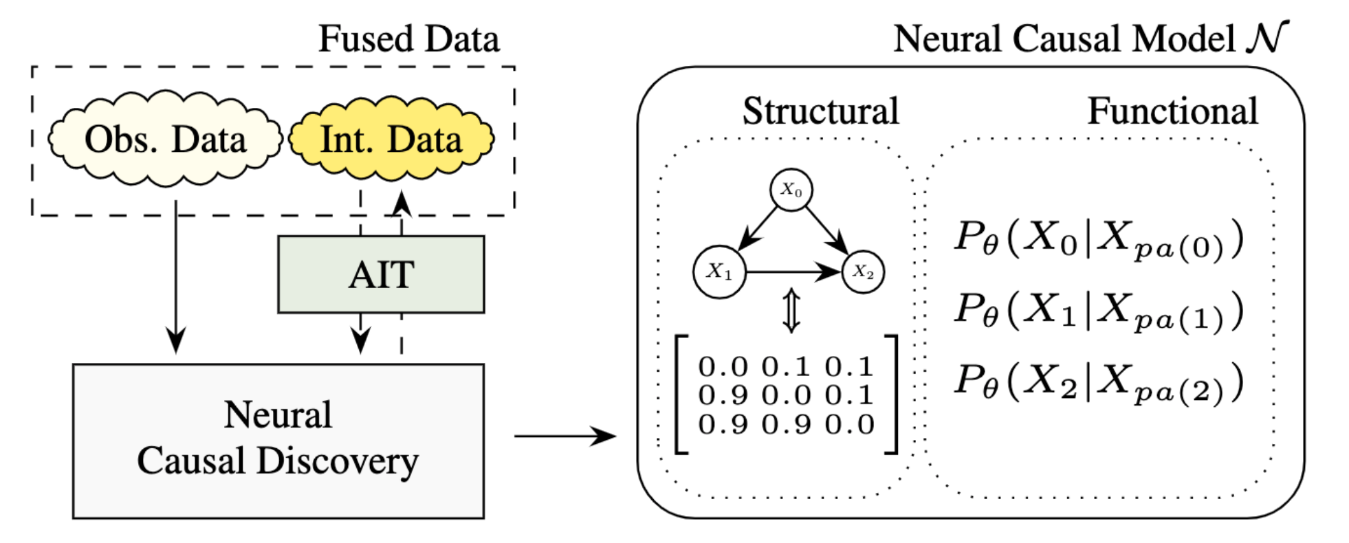
Neural causal discovery from fused data aims at fitting fused data with a neural causal model $\mathcal{N}$, an SCM with smoothly differentiable parameters of functional and structural nature, using a score-based objective. Structural parameters $\gamma$ encode our belief in the underlying graph structure $G$, usually in form of a learned soft-adjacency matrix representing a distribution over graphs. Functional parameters $\theta$ encode the conditional probability distributions (CPDs) $P(X_i|X_{pa(i})$ through neural networks that either learn parameters of a distributional family (e.g. Gaussians or normalizing flows) or approximate the function itself. This is usually realized by a stack of MLPs, i.e. one MLP per variable, to represent its conditional distribution.

• Structure Discovery from Interventions (SDI):
  The SDI framework approach reformulates the problem of causal discovery from fused, discrete data as a discrete optimization problem using neural networks. The framework proposes to learn the parameters of a neural causal model using a two-stage training procedure with alternating phases of optimization.
  
  Functional fitting fits under a fixed structural belief the functional parameters $\theta$ (representing the observational CPDs) to observational data. In order to account for the stochastic nature of the structural belief, the method samples different hypothesized graphs in this stage and uses them in a dropout-like fashion to mask out all variables except the direct causal parents according to the graph while fitting the functional parameters. This enforces the CPDs to be trained on different sets of parents and will converge to the set of true parents as the structure converges.
  
  Structural fitting freezes the functional parameters and evaluates the fit to interventional data of different hypothesized graphs. The adaptation scores are then used to update the belief in the graph structure by propagating them to update the structural parameters. The method performs competitively to many other methods. However, it processes all interventions in a random and independent manner, a strategy that scales poorly to larger graphs.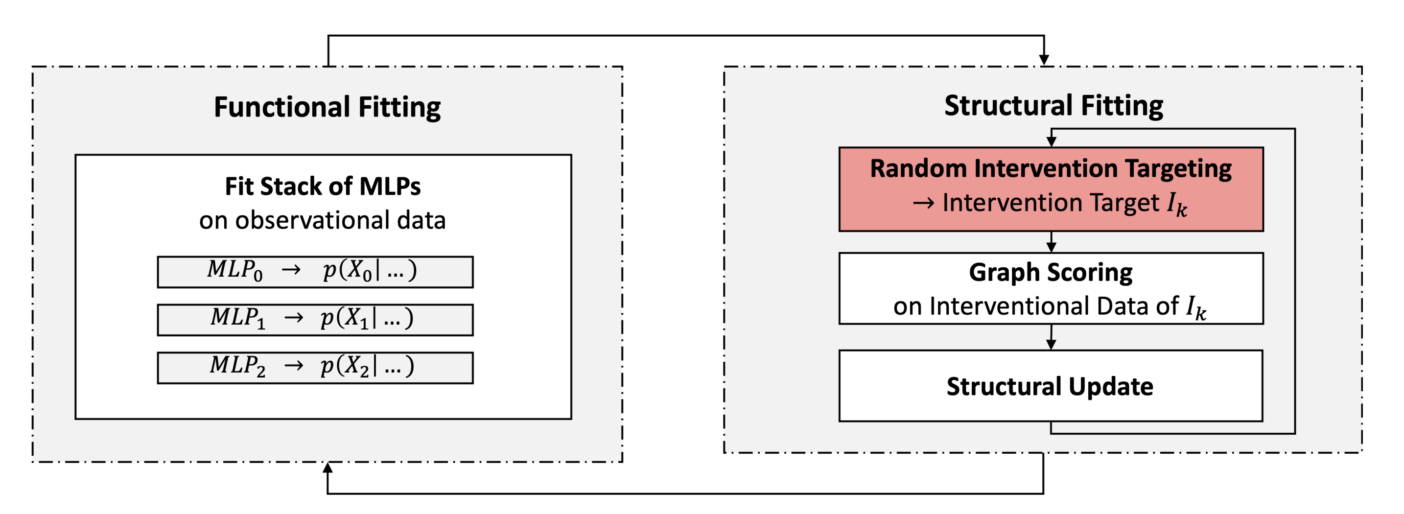
  

How to actively intervene with Active Intervention Targetting (AIT)?

We present a score-based, adaptive intervention design strategy, called AIT, which is applicable to any neural causal discovery method which provides access to structural and functional parameters.

Assumptions: The proposed method does not have to assume causal sufficiency per se. However, it inherits the assumptions of the selected base framework, and this may include causal sufficiency depending on the base algorithm of choice. In case the underlying framework can handle unobserved variables and offers a generative method for interventional samples, then our method is also applicable

A Score for Intervention Targeting

Given a structural belief state $\gamma$ with its corresponding functional parameters $\theta$, and a possible set of intervention targets $I$ (single and multi-node intervention targets), we wish to select the most \textit{informative} intervention target(s) $I_{k^*} \in I$ to identify as quickly as possible the underlying structure. In AIT, we decide where to intervene by computing a score for all possible intervention targets. This score provides us with an estimate how informative an intervention at that target would be with respect to the current evidence.

• We claim that such informative interventions would yield relatively high discrepancies between post-interventional samples drawn under different hypothesis graphs, making it possible to discriminate better among these candidate graphs and indicating larger uncertainty about the intervention target's relation to its parents and/or children.

We thus construct an F-test-inspired score to seek the target $I_{k^*}$ exhibiting the highest discrepancies between post-interventional sample distributions generated by likely graph structures under fixed functional parameters $\theta$. In order to compare sample distributions over different graphs, we distinguish between two sources of variation: variance between graphs VBG and variance within graphs VWG. While VBG characterizes the variance of sample means over multiple graphs, VWG accounts for the sample variance when a specific graph is fixed. %As in SDI and DCDI, We mask the contribution of the intervened variables $I_k$ to VBG and VWG, and construct our discrepancy score $D$ as a ratio: $$ \small D = \frac{\texttt{VBG}}{\texttt{VWG}} $$ This discrepancy score attains high values for intervention targets of particular interest. While VBG itself indicates for which intervention targets the model is unsettled about, an extension to the proposed variance ratio enables more control over the region of interest. Given a fixed set of graphs $\mathcal{G}$ and a fixed interventional sample size across all graphs, let us assume a scenario where multiple intervention targets attain high VBG. Assessing VWG allows us to distinguish between two extreme cases: (a) targets with sample populations that exhibit large VWG, (b) targets with sample populations that exhibit low VWG. While high VBG in (a) might be induced by an insufficient sample size due to high variance in the interventional distribution itself, (b) clearly indicates high discrepancy between graphs and should be preferentially studied.

Computation Details

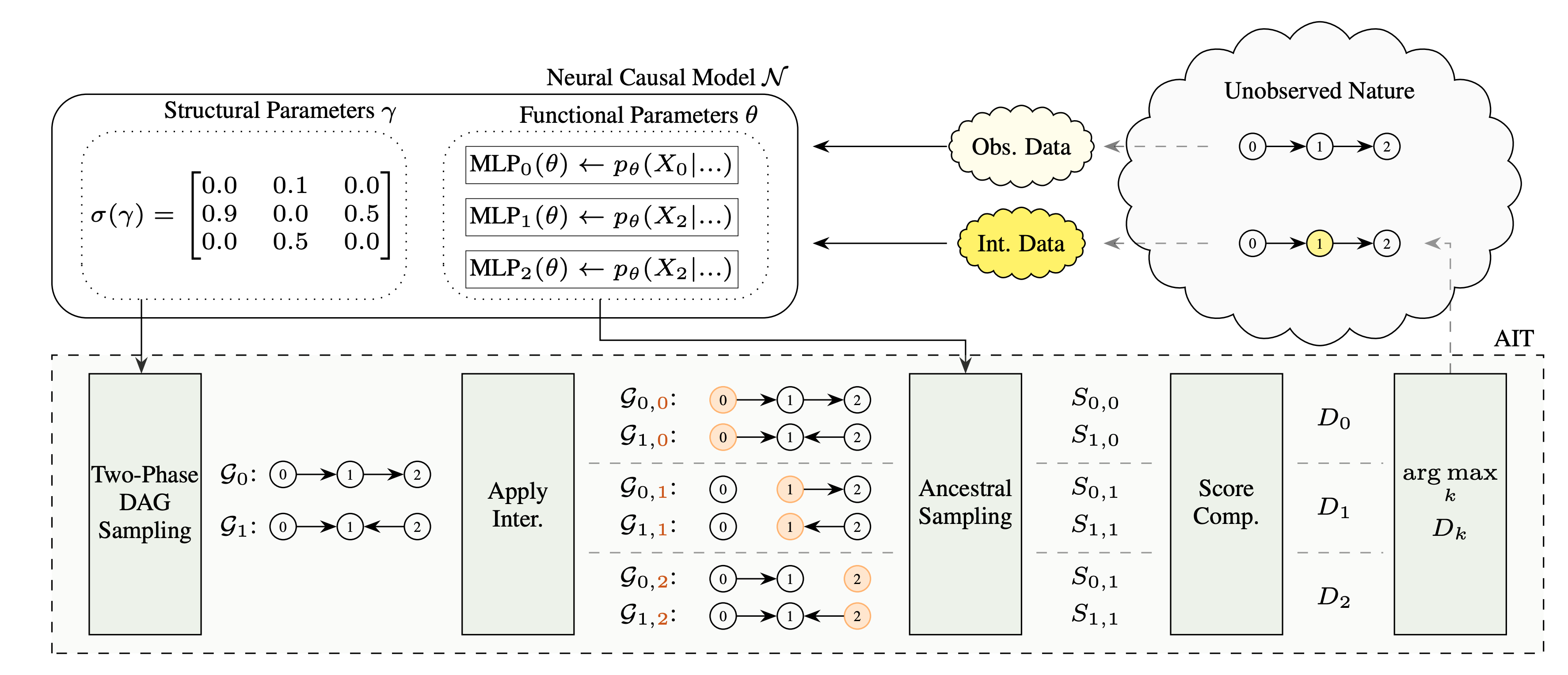
We begin by sampling a set of graphs $\mathcal{G}=\{\mathcal{G}_i\}, \, i = 1,2,3,\ldots$ from our structural parameters $\gamma$. This $\mathcal{G}$ will remain fixed for all considered interventions for the current experimental round. Then, we fix an intervention target $I_k$ and apply the corresponding intervention to $\theta$, resulting in partially altered functional parameters $\theta_k$ where some conditionals have been temporarily changed to be overriden by the intervention. Next, we draw interventional samples $\smash{S_{i,k}}$ from $\theta_k$ on the post-interventional graphs $\mathcal{G}_{i,k} $ (i.e. intervention on target $I_k$ applied to graph $\mathcal{G}_i$). In the variance calculation, we set the variables of the intervention targets $I_k$ to zero to mask off their contribution to the variance. Having collected all samples over the considered graphs for the specific intervention target $I_k$, we compute $\smash{\texttt{VBG}_k}$ and $\smash{\texttt{VWG}_k}$ as follows: \[ \small \begin{split} \texttt{VBG}_k &= \sum_i < \big(\mu_{i,k} - \bar{\mu}_{k}\big), \big(\mu_{i,k} - \bar{\mu}_{k}\big) > \\ \texttt{VWG}_k &= \sum_i \sum_j <\big(\big[S_{i,k}\big]_{j} - \mu_{i,k}\big), \big(\big[S_{i,k}\big]_{j} - \mu_{i,k}\big)> \end{split} \] where $\bar{\mu}_k$ is a vector of the same dimension as any sample in $S$ and denotes the overall sample-mean over all graphs in the interventional setting $I_k$. Further, $\mu_{i,k}$ denotes the mean of samples drawn from graph $\mathcal{G}_{i,k}$ and $\big[S_{i,k}\big]_{j}$ is the $j$-th sample of the $i$-th graph configuration under intervention $I_k$. Finally, we construct the discrepancy score $D_k$ of $I_k$ as: \[ \small D_k \leftarrow \frac{\texttt{VBG}_k}{\texttt{VWG}_k}. \] In contrast to the original definition of the F-Score, we can ignore the normalization constants due to equal group size and degree-of-freedoms.

How to sample DAGs from a soft-adjacency matrix?

We present a scalable two-stage DAG sampling technique for the efficient generation of hypothesis DAGs based on a soft-adjacency matrix, which is a common parametrization of the structural belief.

• Soft-Adjacency Matrix:
  Given a learnable graph structure $\gamma \in \mathbb{R}^{N \times N}$ of a graph over $N$ variables, the soft-adjacency matrix is given as $\sigma(\gamma) \in [0,1]^{N \times N}$ such that $\sigma{(\gamma_{ij})} \in [0,1]$ encodes the probabilistic belief in random variable $X_j$ being a direct cause of $X_i$, where $\sigma(x) = (1+\exp(-x))^{-1}$ denotes the sigmoid function. For the ease of notation, we define $A = \sigma(\gamma)$ and $A_l$ denotes the considered soft-adjacency $\sigma(\gamma)$ at iteration $l$. Note that the shape of $A_l$ changes through the iterations.

Two-Phase DAG sampling

Embedding AIT into recent differentiable causal discovery frameworks requires a graph sampler that generates a set of likely graph configurations under the current graph belief state. However, drawing samples from unconstrained graphs (e.g. partially undirected graphs or cyclic directed graphs) is an expensive multi-pass process. Here, we thus constrain our graph sampling space to DAGs. Since most differentiable causal structure learning algorithms learn edge beliefs in the form of a soft-adjacency matrix, we present a scalable, two-stage DAG sampling procedure which exploits structural information of the soft-adjacency matrix beyond independent edge confidences. More precisely, we start by sampling topological node orderings from an iterative refined score and construct DAGs in the constrained space by independent Bernoulli draws over possible edges. We can thus guarantee DAGness by construction and do not have to rely on expensive, non-scalable techniques such as rejection sampling or Gibbs sampling. The overall method is inspired by topological sorting algorithms of DAGs where we iteratively identify nodes with no incoming edges, remove them from the graph and repeat until all nodes are processed.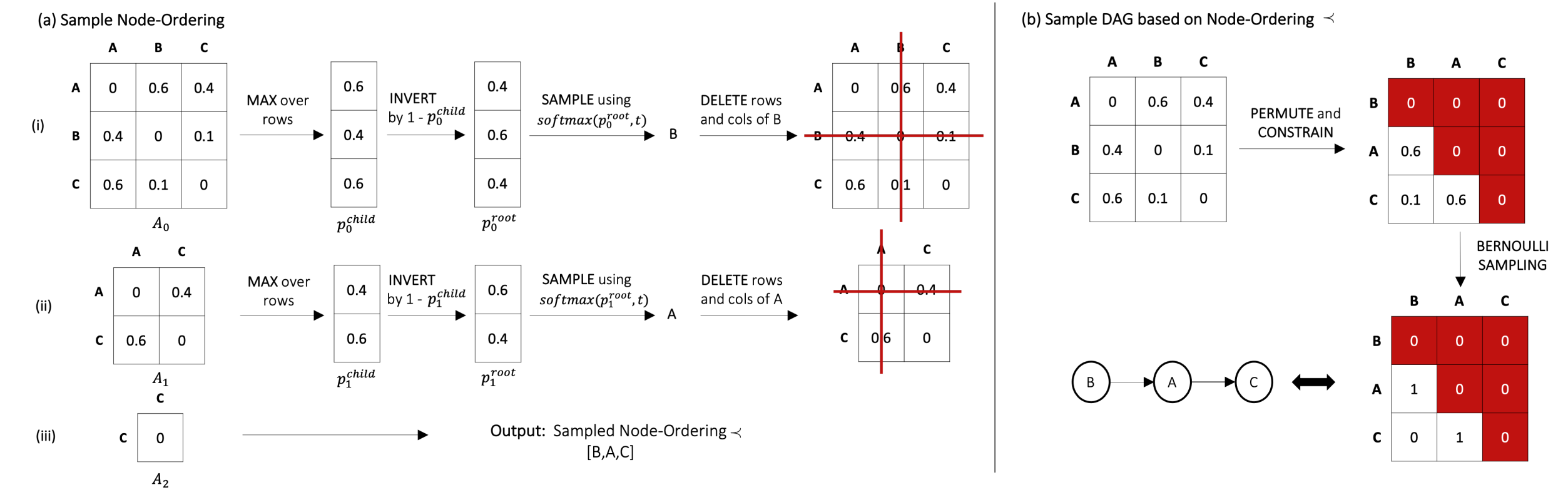

Phase 1: Sample Node Orderings

For the iterative root sampling procedure, we start at iteration $l=0$ with an initial soft-adjacency $A_l = A$ and apply the following routine for $N$ iterations. We take the maximum over rows of $A_l$, resulting in a vector of independent probabilities $p_l^{child}$, where $p_l^{child}(i)$ denotes the maximal probability of variable $X_i$ being a child of any other variable at the current belief state. After taking the complement $p_l^{root} = 1-p_l^{child}$, we arrive at $p_l^{root}$ where $p_l^{root}(i)$ denotes the approximated probability of variable $X_i$ being a root node in the current round. In order to arrive at a normalized distribution to sample a root node, we apply a temperature-scaled softmax: \[ \small p_l(i) = \mathrm{softmax}(p_l^{root}/t)_i = \frac{\exp\big[p_l^{root}(i)/t\big]}{\sum_{j}^{ }\exp\big[p_l^{root}(j)/t\big]} \] where $t$ denotes the temperature. The introduction of temperature-scaling allows to control the distribution over nodes and account for the entropy of the structural belief. We proceed by sampling a (root) node as $r_l \sim Categorical(p_l)$ and delete all corresponding rows and columns from $A_l$ and arrive at a shrinked soft-adjacency $A_{l+1} \in [0,1]^{(N-l-1) \times (N-l-1)}$ over the remaining variables. We repeat the procedure until we have processed all nodes and have a resulting topological node ordering $\prec$ of $[r_0, ..., r_{N-1}]$.

Phase 2: Sample DAGs based on Node Orderings

Given a node ordering $\prec$, we permute the soft-adjacency $A$ accordingly and constrain the upper triangular part by setting values to $0$ to ensure DAGness by construction. Finally, we sample a DAG by independent Bernoulli draws of the edge beliefs.

AIT improves Identifiability and Sample-Efficiency

Improved Structure discovery

We evaluate accuracy in terms of Structural Hamming Distance (SHD) on a diverse set of synthetic non-linear datasets under both SDI and DCDI, adopting their respective evaluation setups. SDI with AIT outperforms all baselines and SDI with random intervention targeting over all presented datasets. It enables almost perfect identifiability on all structured graphs of size 15 except for the $\texttt{full15}$ graph, and significantly improves structure discovery of random graphs with varying densities. As the size or density of the underlying causal graphs increases, the benefit of the selection policy becomes more apparent. We also examine the effectiveness of our proposed method for DCDI on non-linear data from random graphs of size 10. Active Intervention Targeting improves the identification in terms of sample complexity and structural identifiability compared with random exploration. We observe a clear impact of the targeting mechanisms on the order and frequency of interventional targets presented to the model.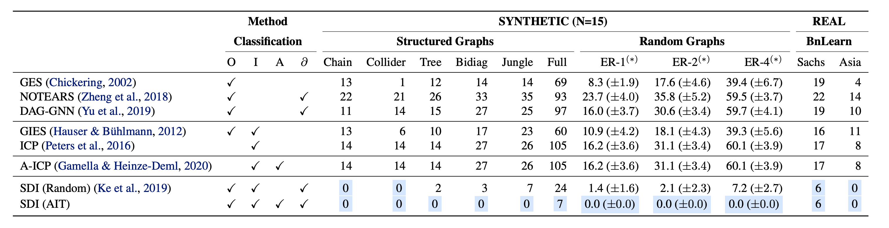

Effect of AIT on Sample-Complexity

Aside from the significantly improved identification of underlying causal structures, our method allows for a substantial reduction in interventional sample complexity. After reaching the ``elbow'' point in terms of structural Hamming distance, random intervention targeting requires a fairly long time to converge to a solution within the MEC. In contrast, our proposed technique continues to select informative intervention targets beyond the elbow point and more quickly converges to the correct graph within the MEC. The continued effectiveness of our method directly translates to increased sample-efficiency and convergence speed, and is apparent for all examined datasets.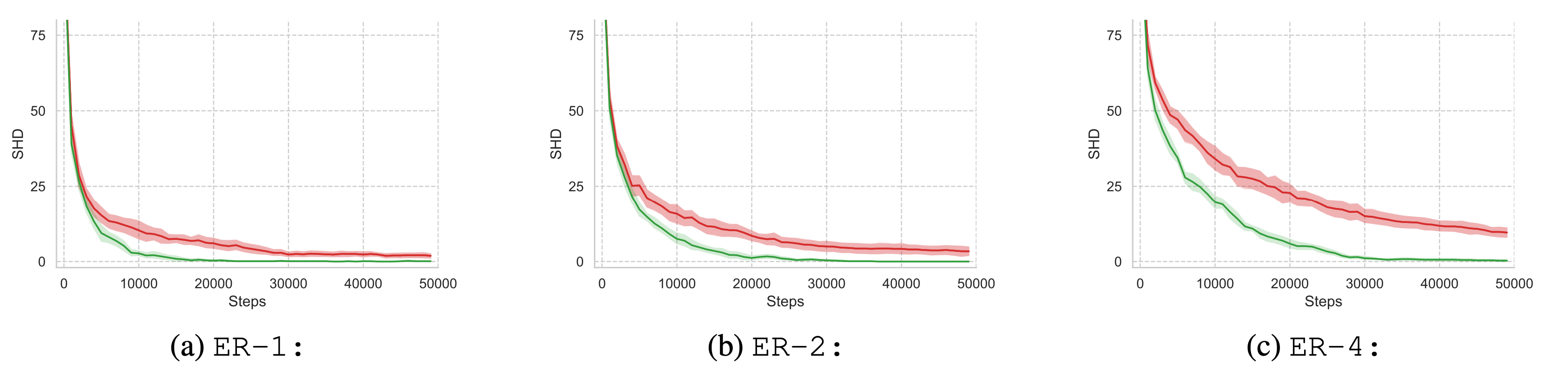

Distribution of selected Intervention Targets

The careful study of the behaviour of the proposed method under our chosen synthetic graphs enable us to reason about the method's underlying dynamics. Analysing the dynamics of intervention targeting reveals that the distribution of target node selections is linked to the topology of the underlying graph. More specifically, the number of selections of a given target node strongly correlates with its out-degree and number of descendants in the underlying ground-truth graph structure. That our method prefers interventions on nodes with greater (downstream) impact on the overall system can be most clearly observed in the distribution of target selection on the example of the synthetic \texttt{jungle} graph .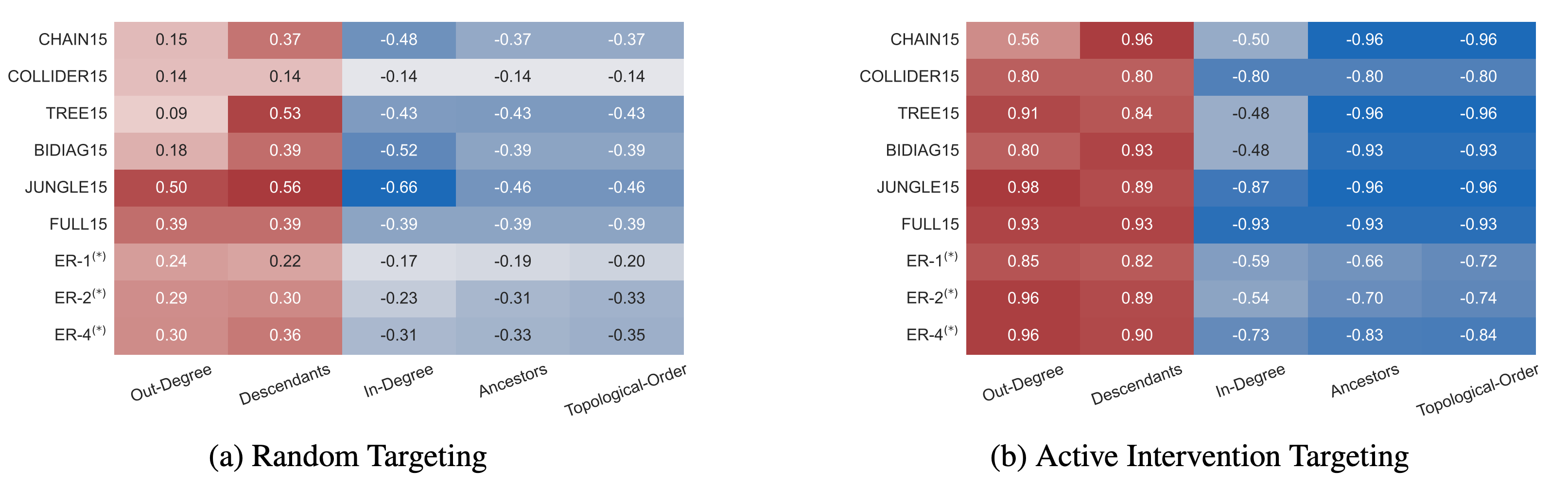

Improved Robustness in Noise-Perturbed Environments

Considering that noise significantly impairs the performance of causal discovery, we examine the performance of active intervention targeting in noise-perturbed environments with respect to SHD and convergence speed and compare it with random intervention targeting. We conduct experiments under different noise levels in the setting of binary data generated from structured and random graphs of varying density. A noise level $\eta$ denotes the probability of flipping a random variable and applying it to all measured variables of observational and interventional samples. Through all examined settings, we observe that active intervention targeting significantly improves identifiability in contrast to random targeting. The observed performance boost is clearly noticeable in the convergence speed. While the convergence-gap gets more significant with an increasing noise level, random targeting does not converge to the ground-truth graphs for all graphs with a noise level higher than $\eta = 0.02$. In contrast, AIT still converges to the correct graph and shows even a convergence tendency for $\eta = 0.05$. These findings support our observation from different experiments that active intervention targeting leads to a more controlled and robust graph discovery.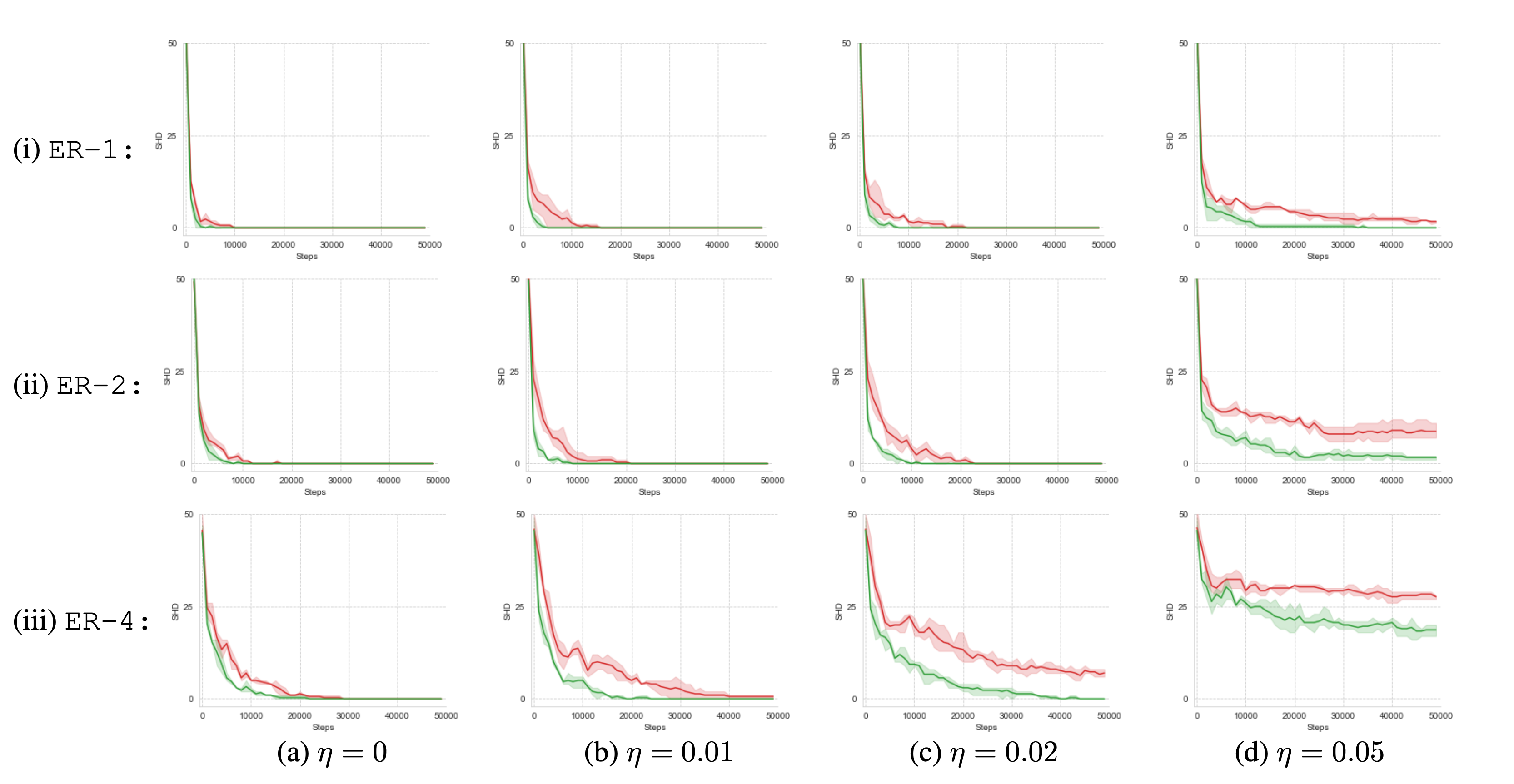

More results coming soon ...

• Site is currently under construction... more results will follow soon!

Promising Results for Further Developments

Promising results have driven the recent surge of interest in differentiable methods for causal structure learning from observational and interventional data. In this work, we augment existing neural causal discovery methods with the ability to actively intervene and propose an active learning method to choose interventions. We show in a systematic empirical study across multiple noise-free and noise-perturbed datasets that active intervention targeting not only improves sample efficiency but also the identification of the underlying causal structures compared to random intervention targeting. Our results indicate that the guided selection of intervention targets leads to a more controlled discovery with favourable properties with respect to the optimization. The increased performance boost for larger graphs is in line with our expectation as random intervention targeting scales poorly to graphs of larger size.